A minimal bonded discrete element model for sea ice
Page still under construction!
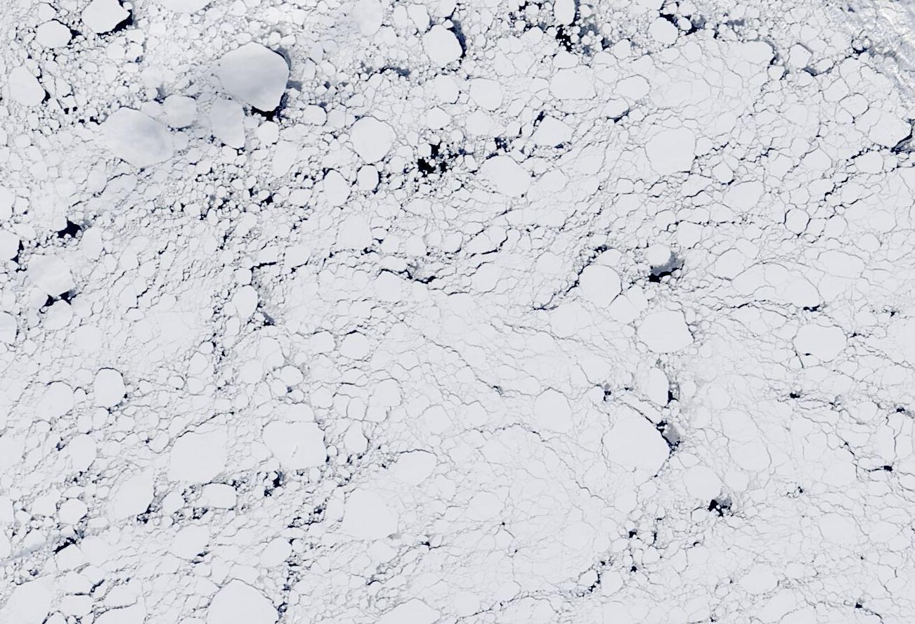
Sea ice is a critical component of the Earth system, mediating ocean heat uptake, driving the global ocean overturning circulation, buffering vulnerable ice shelves from ocean waves, and serving as a key habitat for the primary producers at the bottom of the food chain up through keystone species like the polar bear. Through polar amplification, climate change is impacting the polar regions more than anywhere else in the world. Despite the urgent need for accurate predictions of the future sea ice state, current climate models struggle to reproduce sea ice trends on seasonal and decadal timescales. These models simulate sea ice as a continuous medium despite the discontinuities arising from fracturing and floe-floe interactions. Discrete element models (DEMs) can directly resolve these discontinuities, making them valuable tools for developing parameterizations of subgrid-scale physics to improve the sea ice momentum budget in climate models. Because DEMs resolve interactions between individual discrete elements, they are typically computationally expensive and contain many unconstrained parameters. In this work, we develop, calibrate, and evaluate the performance of a minimal bonded discrete element model for process-based studies, foregoing some physics for a small parameter space and computational efficiency.
TLDR
We adapted a computationally cheap bonded discrete element model in LAMMPS that reproduces localized failure and compressive ice arch formation. Across many simulations, the outcomes fall into four regimes represented by one control parameter.
Why a minimal model?
Discrete-element models can be expensive and parameter-heavy. By intentionally keeping the physics and parameter space small, we can calibrate cleanly and run large ensembles to learn what controls behavior.
What you’ll see below
A figure-first walkthrough: how the DEM works, how damage localizes, how fracture patterns compare across different initial conditions, how ice arches form/collapse, and how the four arch regimes depend on model parameters.
1) What is a discrete-element sea-ice model?
Rather than evolving an equation describing bulk sea ice behavior on a predefined grid, discrete element models solve the equations of motion for each element based on particle interaction rules. By starting with a bonded assembly of particles, fine-scale fractures emerge naturally and no assumptions about continuous fields need to be made.
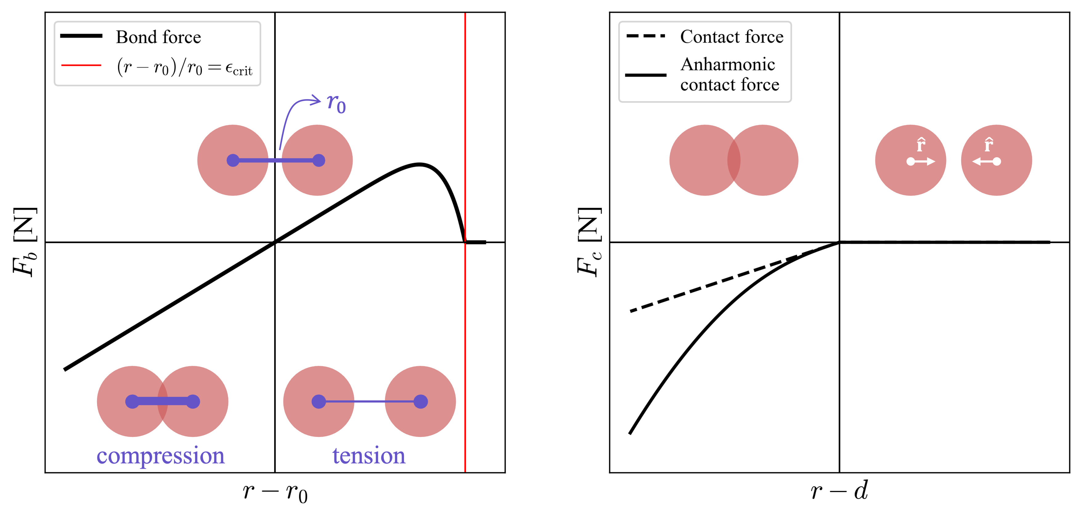
Figure: Bond and contact laws. Bonds resist deformation and fail in tension when the strain exceeds a critical value, while contacts transmit compressive forces during collisions.
2) The size effect
Larger materials are weaker due to a heightened probability of weaker defects, known as the statistical size effect. Similarly, discrete element simulations with few elements will be stronger than those with more elements, but this influence is expected to plateau at some granularity: the ratio of element size to domain size.
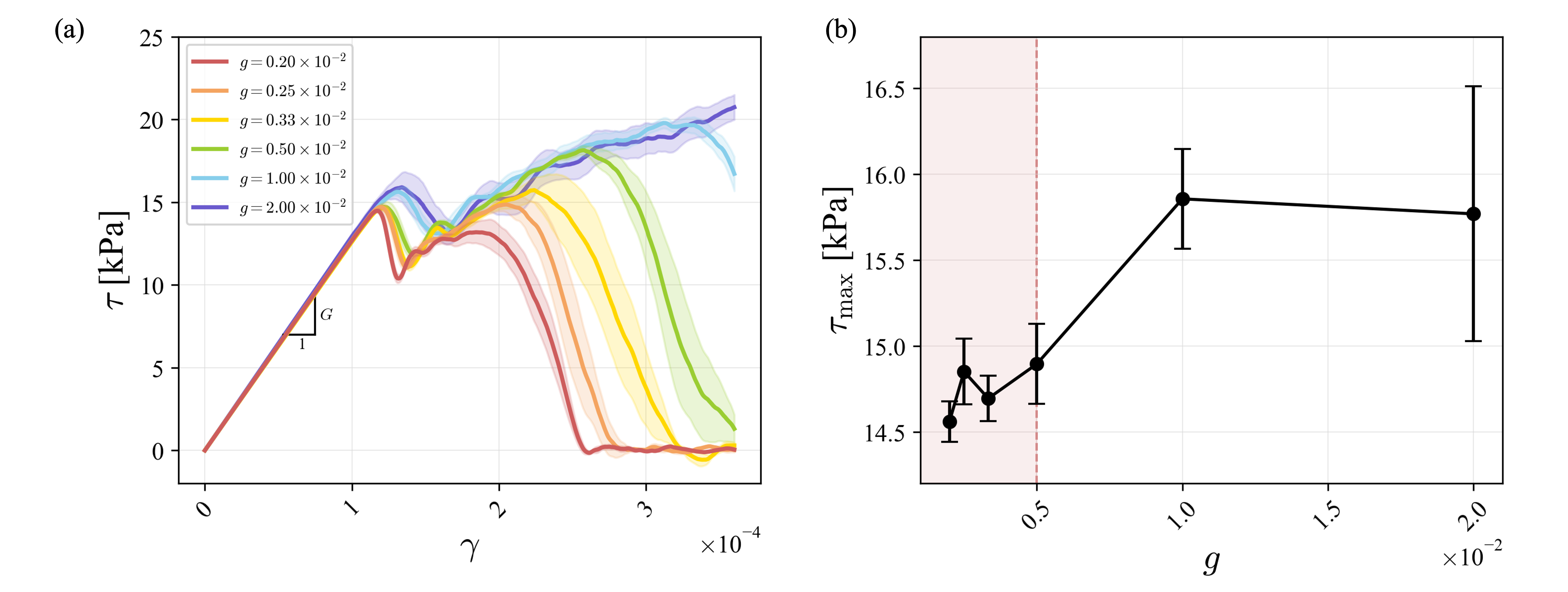
Figure: (a) Ensemble-averaged shear stress–strain responses for varying granularity. (b) Peak shear stress as a function of granularity. The red shaded region is our chosen granularity threshold to minimize the influence of the size effect. For subplots (a) and (b) shaded regions and error bars, respectively, indicate the standard error across five ensemble members per granularity, each initialized from a distinct random particle packing.
2) Deformation localized in space and time under low strain rate.
Sea ice deformation is localized and intermittent. Here, we run a simple shear simulation which reveals that our simple model creates ice that shares these same deformation characteristics.
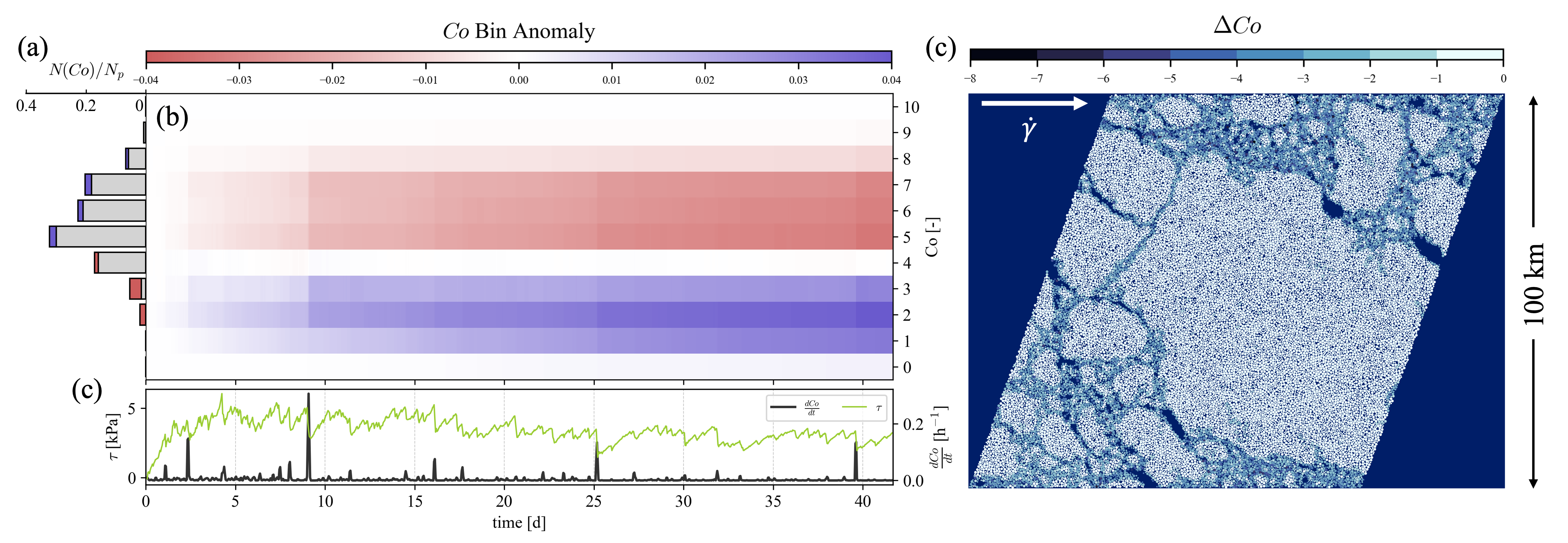
Figure: (a) Histogram time series illustrating how bond breaking occurs in isolated events. (b) Time series of the damage rate (black) corresponding with peaks in shear stress (green). (c) The total change in coordination number for each particle at the end of the 43 day simulation.
3) Ice arch formation and collapse
In a canonical experiment, northerly wind speeds are increased linearly over 36 hours.
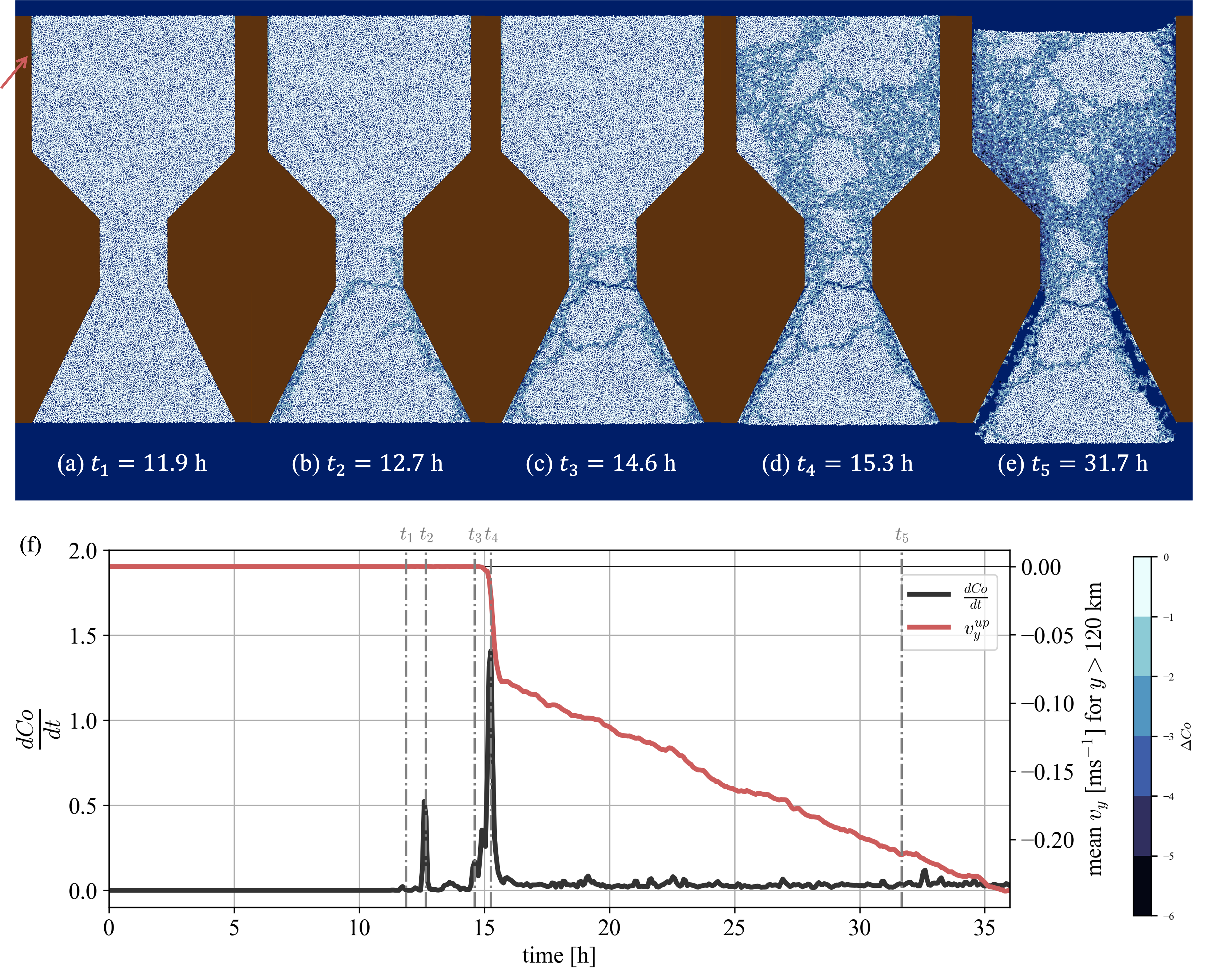
Figure: [text]
4) Regimes as functions of internal parameters from idealized channel simulations
[text]
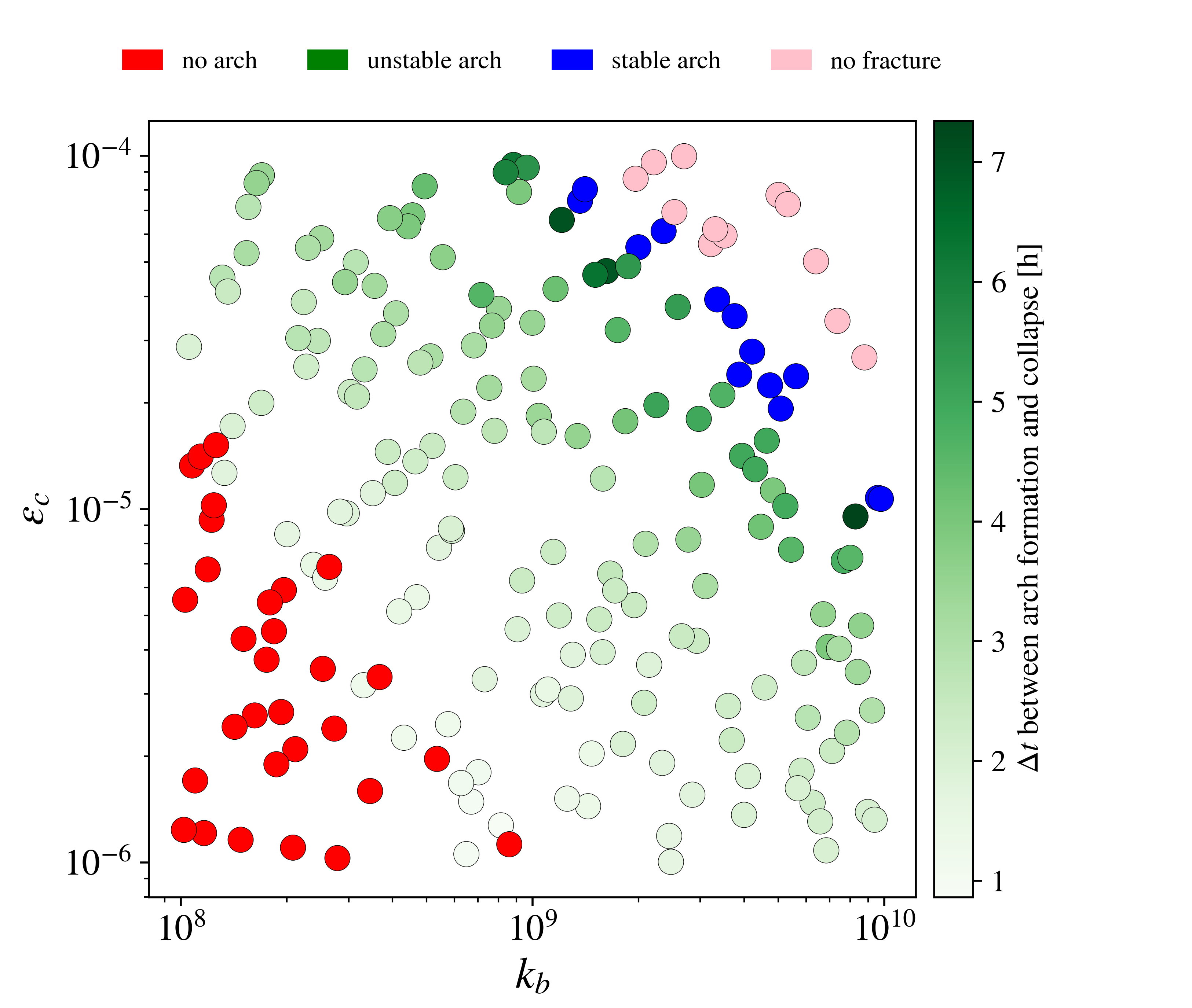
Figure: [text]